RF Workbench
Browser RF tools on this site. Draw a signal chain and get a live cascade of gain, noise figure, IP3, P1dB and sensitivity; load Touchstone files and compare parts on rectangular or Smith axes. Nothing is uploaded.
This page’s tools are the ones I’d otherwise open three separate programs for. They run entirely in the browser, so a Touchstone file you drop in never leaves your machine.
Signal chain and cascade
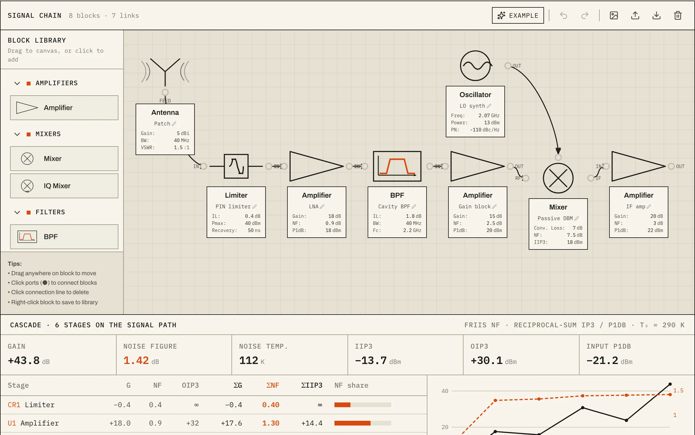
The block-diagram editor started as rfblock, a drag-and-drop RF diagram tool I prototyped in Lovable. It could draw a chain but calculated nothing. I ported it into this site’s design system and added the analysis it was missing:
- A cascade engine with Friis noise figure at 290 K, equivalent noise temperature, reciprocal-sum IP3 and P1dB, and receiver figures for any bandwidth: kTB noise floor, sensitivity at a required SNR, and spur-free dynamic range.
- RF-correct block mapping. A matched passive’s noise figure equals its loss. An N-way splitter charges 10·log₁₀N plus insertion loss along one branch. A mixer’s gain is minus its conversion loss, with NF defaulting to the conversion loss when none is given. Antennas and oscillators aren’t stages.
- A signal-path finder that works from port roles rather than the order you clicked the wires. It starts at a receive antenna, never follows the LO into the signal path, and picks a branch at splitters and switches.
The example chain is the same one drawn in Fig. 1 on the home page, and the test suite checks that both give 43.8 dB and 1.42 dB.
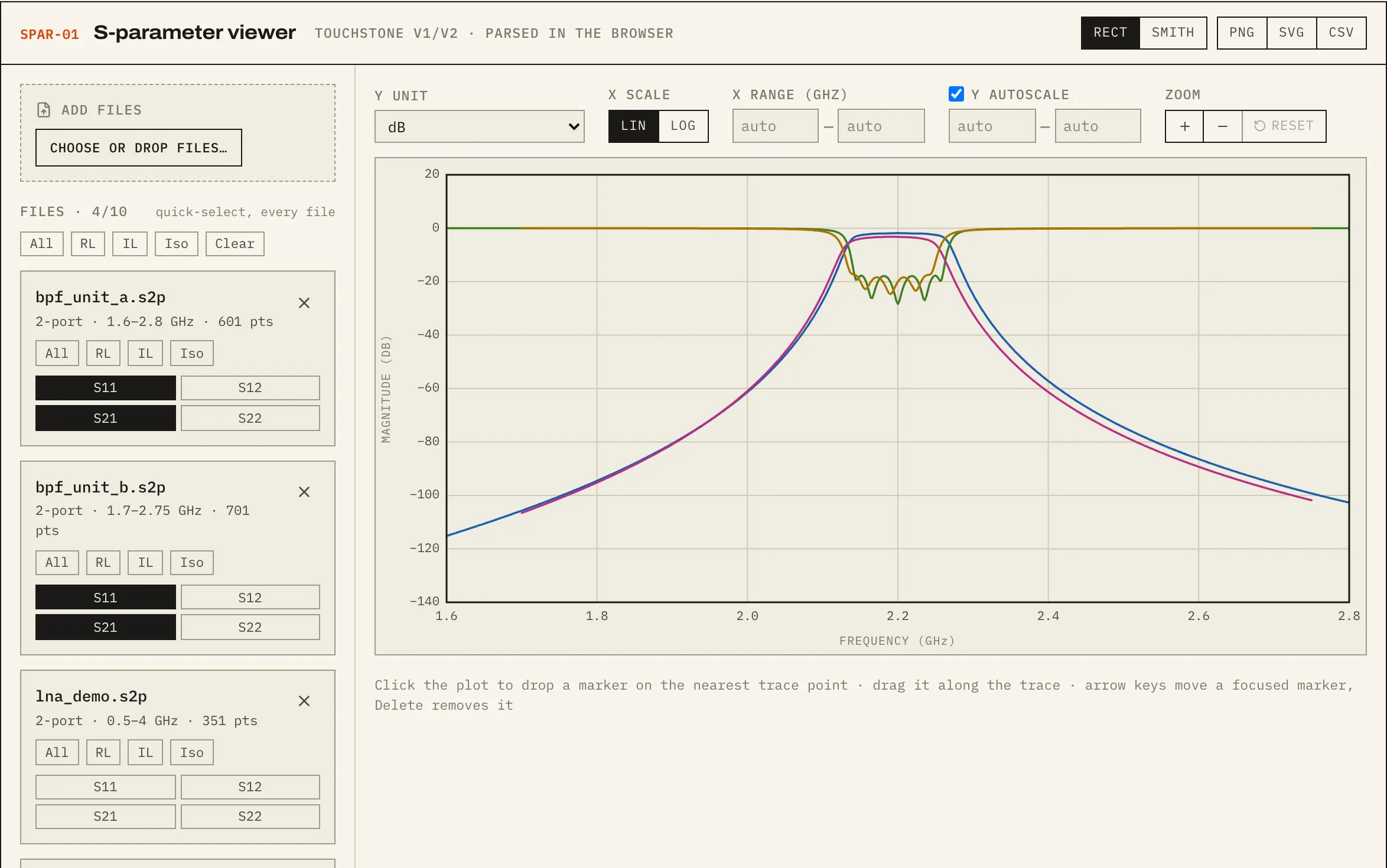
S-parameter viewer
A client-side rebuild of my S-parameter viewer, which originally needed a Python backend:
- A Touchstone v1 and v2 parser, written to match scikit-rf’s behaviour: free-form number streams, the 2-port v1 S21/S12 ordering quirk, v2 matrix formats, and noise blocks detected and skipped.
- Six Y units: dB, linear, wrapped phase, unwrapped phase, VSWR and group delay. The last three are new compared with the original tool.
- Cross-grid trace math that interpolates magnitude and unwrapped phase separately. Interpolating raw real and imaginary parts across a phase rotation invents magnitude dips.
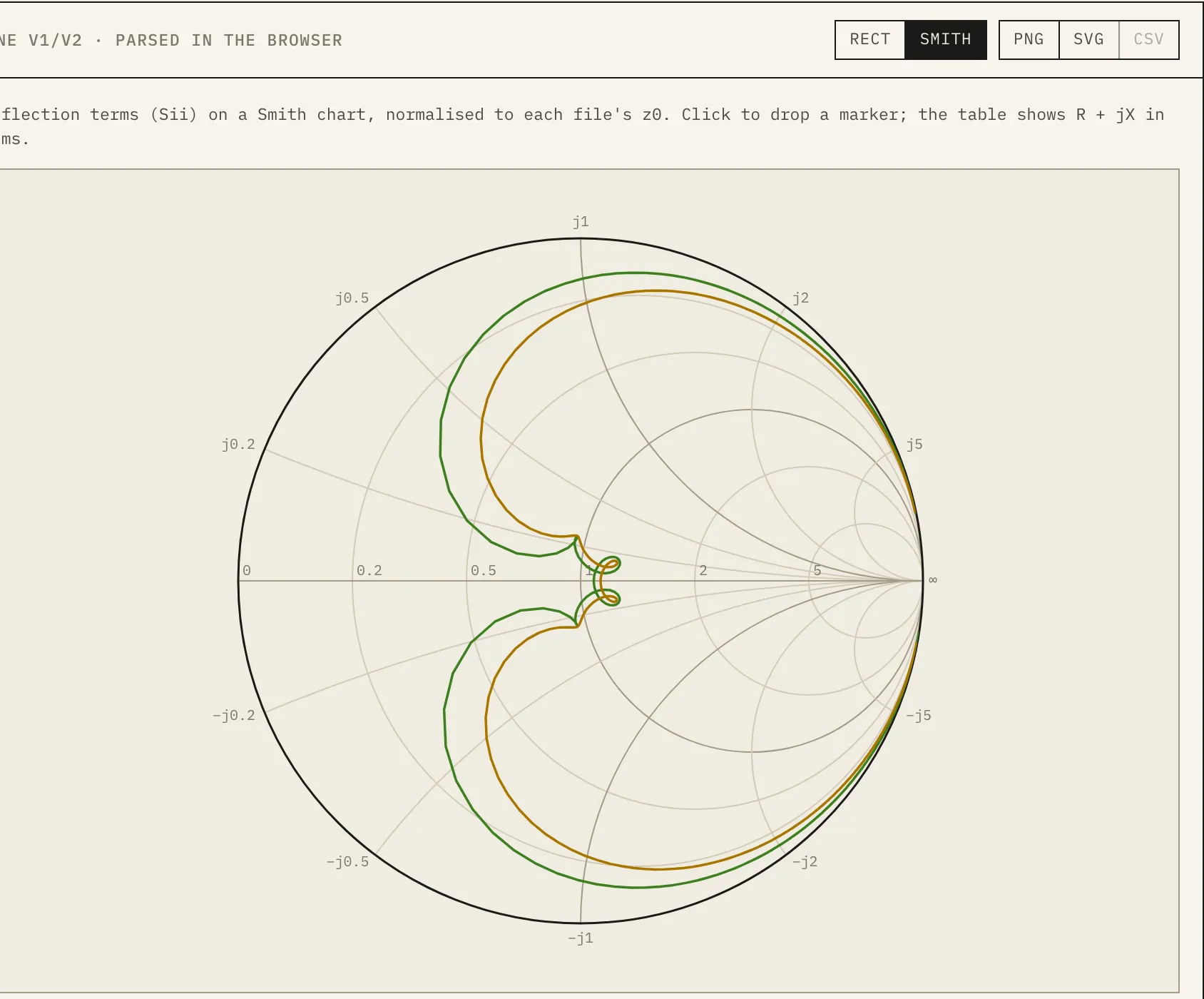
- A Smith chart with markers showing R + jX in ohms.
- Snap-to-point markers, and PNG, SVG and CSV export.
The demo parts are synthetic. A short Python script computes them from circuit models: a lumped 5-pole Chebyshev bandpass with finite-Q resonators, an LNA, and a series-RLC patch antenna. No real part’s data is on this site.
How it was built
The work split cleanly by interface, so I wrote specs for two agents and ran them in parallel with the port:
- Cascade engine agent: the exact function signatures, the RF conventions, and a rule that tests be derived by hand, not by calling the code under test. It came back with 104 tests, and it also corrected my spec on the P1dB formula.
- Viewer agent: the parsing rules, the math, the design system, and a required visual check. It rendered the viewer in both themes and at phone width and fixed what it saw before reporting.
- Me: porting the editor, wiring the cascade panel, generating the demo data, and reviewing both agents’ work before it merged.